Parallel Folds: Reducers, Tesser and Linear Regression
In this article, extracted from Chapter 5, Clojure for Data Science, I'll show some principles of efficient big data analysis and how they can be applied using Clojure. I'll be using three Clojure libraries: reducers, Iota, and Tesser to show how the calculation of statistics can be scaled to very large volumes of data through parallelism and by avoiding unneccessary iterations over the data.
By the end of this article you'll be able to build a predictive model using linear regression. Linear regression is a machine learning algorithm that attempts to learn a linear relationship between a single output (usually called the dependent variable) and one or more inputs (often called the independent variables). We'll be using data from the U.S. Internal Revenue Service (IRS) on ZIP code-level statistics of income, and attempt to learn a simple linear relationship between two variables: the "salaries and wages" and "unemployment compensation" figures.
Download the code and data
All the code is contained in the example project at https://github.com/clojuredatascience/ch5-big-data. If you'd like to follow along with any of the examples, clone this repository to your local machine.
Download the data
The IRS data I'll use for the examples contains selected income and tax items classified by state, ZIP code, and income classes. It's 100MB in size and should be downloaded from http://www.irs.gov/pub/irs-soi/12zpallagi.csv to the example code's data directory. Since the file contains the IRS Statistics of Income we've renamed the file to "soi.csv" for the examples.
If you're running *nix or OS X, there's a little shell script in the project which will download and rename the data for you. Run it on the command line within the project's directory like this:
script/download-data.sh
Alternatively, if you're on Windows or would prefer to follow manual instructions:
- Download
12zpallagi.csvinto the sample code'sdatadirectory using the link above - Rename the file
12zpallagi.csvtosoi.csv
Running the examples
The example project contains a namespace called cljds.ch5.examples. Each example below is a function in this namespace that you can run in one of two ways: either from the REPL or on the command line, with Leiningen. If you'd like to run the examples in the REPL execute:
lein repl
on the command line. By default the REPL will open in the examples namespace and you can type the code you want to evaluate.
Alternatively, to run a specific numbered example you can execute:
lein run –-example 5.1
or the pass the single-letter equivalent:
lein run –e 5.1
This will run the function named ex-5-1. If you've followed the instructions above to download the data, you should now be able to run the examples.
Inspect the data
Take a look at the column headings in the first line of the file. One way to do this is to load the file into memory, split on newline characters, and take the first result. The Clojure core library function slurp will return the whole file as a string, split in the clojure.string namespace can chop the contents into lines based on the newline character, and first will return line 1:
(require '[clojure.string :as str])

(defn ex-5-1 []
  (-> (slurp "data/soi.csv")
      (str/split #"\n")
      (first)))
The file is around 100MB in size on disk. When loaded into memory and converted to object representations the data will occupy more space. This is incredibly wasteful when we're only interested in the first row.
Fortunately we don't have to load the whole file into memory if we take advantage of Clojure's lazy sequences. Instead of returning a string representation of the contents of the whole file, we could return a reference to the file and then step through it one line at a time:
(require '[clojure.java.io :as io])

(defn ex-5-2 []
  (-> (io/reader "data/soi.csv")
      (line-seq)
      (first)))
In the above code we're using clojure.java.io/reader to return a reference to the file and using the core function line-seq to return a lazy sequence of lines from the file. In this way we can read files even larger than available memory one line at a time.
The second approach is a much more efficient way of fetching the column headings. They're replicated below:
"STATEFIPS,STATE,zipcode,AGI_STUB,N1,MARS1,MARS2,MARS4,PREP,N2,NUMDEP,A00100,N00200,A00200,N00300,A00300,N00600,A00600,N00650,A00650,N00900,A00900,SCHF,N01000,A01000,N01400,A01400,N01700,A01700,N02300,A02300,N02500,A02500,N03300,A03300,N00101,A00101,N04470,A04470,N18425,A18425,N18450,A18450,N18500,A18500,N18300,A18300,N19300,A19300,N19700,A19700,N04800,A04800,N07100,A07100,N07220,A07220,N07180,A07180,N07260,A07260,N59660,A59660,N59720,A59720,N11070,A11070,N09600,A09600,N06500,A06500,N10300,A10300,N11901,A11901,N11902,A11902"
This is a wide file! There are 77 columns overal, so we won't identify them all. The key fields we'll be interested in are:
- N1: The number of returns
- A00200: The salaries and wages amount
- A02300: The unemployment compensation amount
If you're curious about what else is contained in the file, the IRS data definition document is available at http://www.irs.gov/pub/irs-soi/12zpdoc.doc.
Counting the records
Our file is certainly wide, but is it tall? Let's see how many rows there are in the file. Having created a lazy sequence this is a simple matter of counting the length of the sequence.
 (defn ex-5-3 []
  (-> (io/reader "data/soi.csv")
      (line-seq)
      (count)))
The above example returns 166,905 including the header row, so we know there are actually 166,904 rows in the file.
The function count is the simplest way to count the number of elements in a sequence. For vectors (and other types implementing the Counted interface) this is also the most efficient, since the collection already knows how many elements it contains and therefore doesn't need to recalculate it. For lazy sequences however, the only way to determine how many elements are contained in the sequence is to step through it from beginning to end.
Clojure's implementation of count is written in Java, but it can be pictured as a reduce over the sequence like this:
(defn ex-5-4 []
  (->> (io/reader "data/soi.csv")
       (line-seq)
       (reduce (fn [i x]
                 (inc i)) 0)))
The function we pass to reduce above accepts a counter i and the next element from the sequence, x. For each x we simply increment the counter i. The reduce function accepts a 'initial value' of zero which represents the concept of 'nothing'. If there are no lines to reduce over, zero will be returned.
As of version 1.5, Clojure offers the Reducers library (http://clojure.org/reducers) which provides an alternative way of performing reductions that trades memory efficiency for speed.
The reducers library
The function we implemented above to count the records is a sequential algorithm. Each line is processed one-at-a-time until the sequence is exhausted. But there's nothing about the operation that demands it be done like this: we could split the number of lines into two sequences (ideally of roughly equal length) and reduce over each sequence independently. When we're done, we would just add together the total number of lines from each sequence together to get the grand total number of lines in the file.
If each reduce ran on its own processing unit then the two count operations could be run in parallel. If we ignore the cost of splitting and recombining the sequences (which we can't, but it's often small compared to the work of the reduction itself), the algorithm could run twice as fast.
This is one of the aims of reducers: to bring the benefit of parallelism to algorithms implemented on a single machine by taking advantage of multiple cores.
Parallel folds with reducers
The parallel version of reduce implemented by the reducers library is called fold. To construct a fold, we have to supply a combiner function (in addition to the reducer function) that will take the results of our reduced sequences (the partial row counts) and return the grant total result. Since our row counts are numbers, the combiner function is simply +.
The previous example, adjusted to use clojure.core.reducers as r, looks like this:
(require '[clojure.core.reducers :as r])

(defn ex-5-5 []
  (->> (io/reader "data/soi.csv")
       (line-seq)
       (r/fold + (fn [i x]
                   (inc i)))))
The combiner function, +, has been included as the first argument to fold and our unchanged reduce function is supplied as the second argument. We no longer need to pass the initial value of zero: fold will get the initial value by calling the combiner function with no arguments. Our example above works because + called with no arguments already returns zero:
(defn ex-5-6 []
  (+))

;; 0
We can visualize the process of seeding the computation with an identity value, iteratively reducing over the sequence of $xs$, and combining the reductions into an output value as a tree:
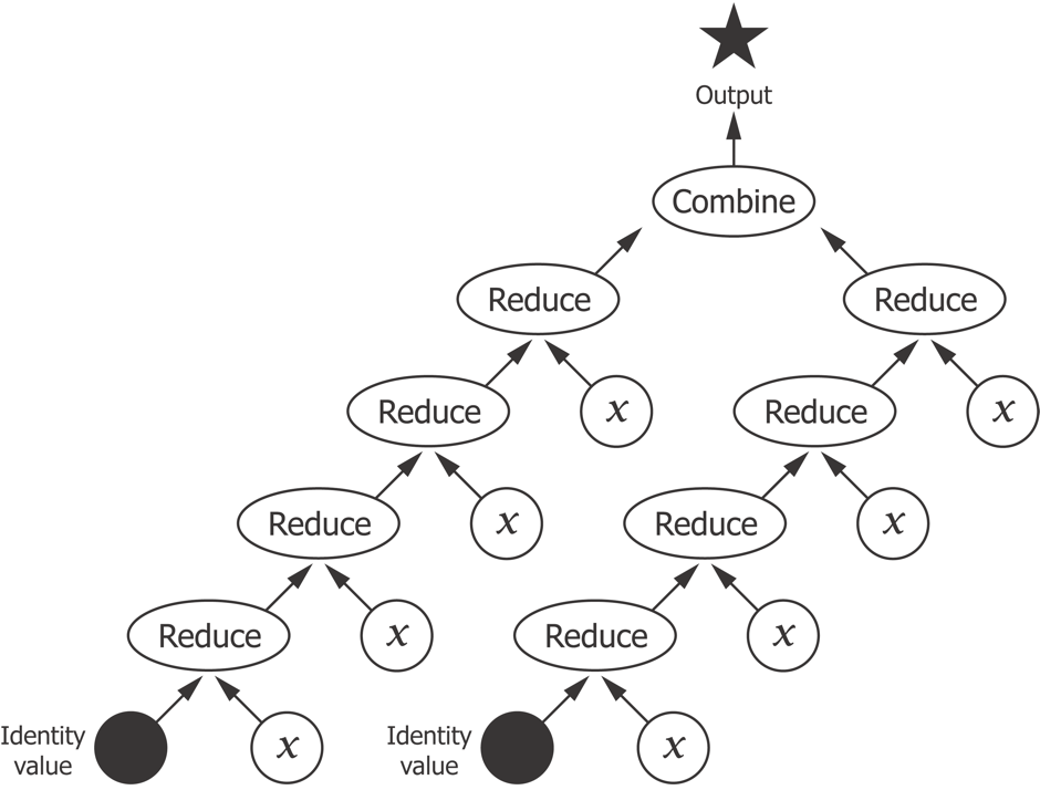
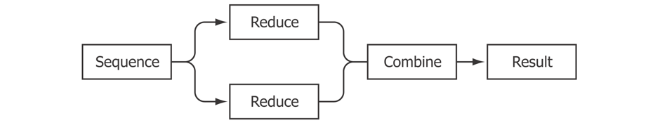
There may be more than two reductions to combine, of course, and in fact the default implementation of fold will split the input collection into chunks of 512 elements. Our 166,000-element sequence will therefore generate 325 reductions to be combined. We're going to run out of page real estate quite quickly with a tree representation diagrams, so let's instead visualize the process more schematically: as a two-step reduce and combine process.
The first step performs a parallel reduce across all the chunks in the collection. The second step performs a serial reduce over the intermediate results to arrive at the final result:
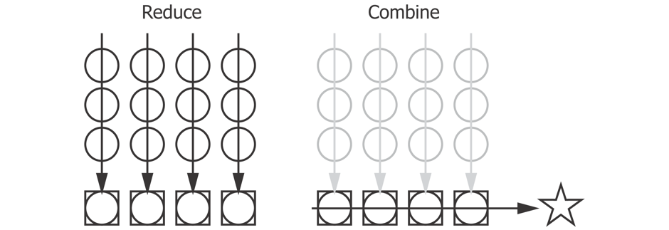
The preceding diagram shows a reduce over a several sequences of $xs$ in parallel, represented as circles, into a series of outputs, represented as squares. The squares are then combined serially to produce the final result, represented by a star.
Loading large files with Iota
Calling fold on a lazy sequence requires Clojure to realize the sequence into memory, and then chunk the sequence into groups for parallel execution. For situations where the calculation performed on each row is small, the overhead involved in this coordination outweighs the benefit of parallelism. We can improve the situation slightly by using a library called Iota (https://github.com/thebusby/iota).
The Iota library loads files directly into data structures suitable for folding over with reducers and can handle files larger than available memory by making use of memory-mapped files. With Iota in place of our line-seq function our line count function becomes:
(require 'iota)

(defn ex-5-7 []
  (->> (iota/seq "data/soi.csv")
       (r/fold + (fn [i x]
                   (inc i)))))
So far we've just been working with sequences of unformatted lines, but if we're going to do anything more than count the rows we'll want to parse them into a more useful data structure. This is another area Clojure's reducers can help make our code more efficient.
Create a reducers processing pipeline
We already know (from the header row) that the file is comma-separated, so let's first create a function to turn each row into a vector of fields. All fields but the first two contain numeric data, so let's parse them into doubles while we're at it:
(defn parse-double [x]
  (Double/parseDouble x))

(defn parse-line [line]
  (let [[text-fields double-fields] (->> (str/split line #",")
                                         (split-at 2))]
    (concat text-fields
            (map parse-double double-fields))))
We'll use the reducers version of map to apply our parse-line function to each of the lines from the file in turn:
(defn ex-5-8 []
   (->> (iota/seq "data/soi.csv")
        (r/drop 1)
        (r/map parse-line)
        (r/take 1)
        (into [])))

;; [("01" "AL" 0.0 1.0 889920.0 490850.0 ...)]
The final into converts the reducers' internal representation (a reducible collection) into a Clojure vector. The previous example should return a sequence of 77 elements representing each column the first row of the file after the header.
We're just dropping the column names at the moment, but it would be great if we could make use of these to return a map representation of each record associating the column name with the field value. The keys of the map would be the column headings and the values would be the parsed fields. The core library function zipmap will create a map out of two sequences: one for the keys and another for the values:
(defn parse-columns [line]
  (->> (str/split line #",")
       (map keyword)))

(defn ex-5-9 []
  (let [data (iota/seq "data/soi.csv")
        column-names (parse-columns (first data))]
    (->> (r/drop 1 data)
         (r/map parse-line)
         (r/map (fn [fields]
                  (zipmap column-names fields)))
         (r/take 1)
         (into []))))
[{:N2 1505430.0, :A19300 181519.0, :MARS4 256900.0 ...}]
A great thing about Clojure's reducers is that in the above computation calls to r/map, r/drop and r/take are compiled into a reduction that's performed in a single iteration over the data. This becomes particularly valuable as the number of operations increases.
For example, let's assume we'd also like to filter out zero ZIP codes. We could extend the reducers pipeline like this:
(defn ex-5-10 []
  (let [data (iota/seq "data/soi.csv")
        column-names (parse-columns (first data))]
    (->> (r/drop 1 data)
         (r/map parse-line)
         (r/map (fn [fields]
                  (zipmap column-names fields)))
         (r/remove (fn [record]
                     (zero? (:zipcode record))))
         (r/take 1)
         (into []))))
The r/remove step is now also being run together with the r/map, r/drop and r/take calls. As the size of data increases it becomes increasingly important to avoid making multiple iterations over the data unnecessarily. Using Clojure's reducers ensures that our calculations are compiled into just a single iteration.
Curried reductions with reducers
To make it clearer to see what's going on we can create a curried version of each of our above steps: to parse the lines, create a record from the fields, and filter zero ZIP codes. The curried version of the function is a reduction "waiting for a collection":
(def line-formatter
  (r/map parse-line))

(defn record-formatter [column-names]
  (r/map (fn [fields]
           (zipmap column-names fields))))

(def remove-zero-zip
  (r/remove (fn [record]
              (zero? (:zipcode record)))))
In each case we're calling one of reducers' functions but without providing a collection to reduce over. The result is a function that can be applied to the collection at a later time, or composed together into a single parse-file function using comp:
(defn load-data [file]
  (let [data (iota/seq file)
        column-names  (parse-columns (first data))
        parse-file (comp remove-zero-zip
                         (record-formatter column-names)
                         line-formatter)]
    (parse-file (rest data))))
It's only when the parse-file function is called with a sequence, as in the last line of the preceding example, that the pipeline is actually executed.
Statistical folds with reducers
With the data parsed it's time to perform some descriptive statistics. Let's assume we'd like to know the average number of returns (column N1) submitted to the IRS by ZIP code. One way of doing this is to add up the values and divide by the count. Our first attempt might look like this:
(defn ex-5-11 []
  (let [data (load-data "data/soi.csv")
        xs (into [] (r/map :N1 data))]
    (/ (reduce + xs)
       (count xs))))

;; 853.37
While this works, it's comparatively slow. We iterate over the data once to create the xs, a second time to calculate the sum using reduce and a third time to calculate the count. The bigger our dataset gets, the larger the time penalty we'll pay for this repetition.
Ideally, we'd be able to calculate the mean value in a single iteration over the data, just like our parse-file function above (even better if we can perform it in parallel, too).
Associativity
Before we proceed, it's useful to take a moment to reflect on why the following code wouldn't do what we want:
(defn mean
  ([] 0)
  ([x y] (/ (+ x y) 2)))
The mean function we've just defined is a function of two arities. This means that it has two different implementations and which is actually called depends on the number of arguments provided when the function is called. Without any arguments it returns 0 (the identity for the mean computation) and with two arguments it returns their mean.
(defn ex-5-12 []
  (->> (load-data "data/soi.csv")
       (r/map :N1)
       (r/fold mean)))

;; 930.54
mean function and produces a different result. Which is correct?Well, if we could expand out the computation in the preceding example for the first three xs, we might see something like the following:
(mean (mean (mean 0 a) b) c)
This isn't the calculation we want to perform. In essence, each time we call mean with the results of a previous mean, we're taking "an average of an average". Technically speaking this is a bad idea because the mean function is not associative. For an associative function, the following equality holds true:
$$ f(f(a,b),c)=f(a,f(b,c)) $$
Addition and subtraction are associative but multiplication and division are not, so the mean function is not associative either. Contrast the mean function usage with the following using +:
(+ 1 (+ 2 3))
which yields an identical result to:
(+ (+ 1 2) 3)
It doesn't matter how we group the sub-calculations with + because addition is associative. Associativity is an important property of functions used with fold because, by definition, the results of a previous calculation are treated as inputs to the next.
The easiest way to calculate the mean in an associative way is to calculate the sum and the count separately. Since both the sum and the count can be calculated with +, they're associative and can be calculated in parallel over the data with fold.
The mean can then be calculated as the very last step simply by dividing one by the other.
Calculating the mean using fold
We'll create a fold to calculate the mean with two custom functions, mean-combiner and mean-reducer. This requires defining three entities:
- The identity value for the fold
- The reducer function
- The combiner function
We discovered the benefits of associativity in the previous section, and so we'll want to update our intermediate mean using only associative operations by calculating the sum and the count separately. One way of representing the two values is a map of two keys, the :sum and the :count. The value that represents the identity for our mean would be a sum of zero and a count of zero, or a map such as the following: {:sum 0 :count 0}.
The combine function, mean-combiner, returns the identity value when it's called without arguments. The two-argument combiner needs to add together the :count and the :sum for each of the two arguments. We can achieve this by merging the maps with +:
(defn mean-combiner
  ([] {:count 0 :sum 0})
  ([a b] (merge-with + a b)))
The mean-reducer function needs to accept an accumulated value (either an identity value or the results of a previous reduction) and incorporate the new x. We do this simply by incrementing the count and adding x to the accumulated sum:
(defn mean-reducer [acc x]
  (-> acc
      (update-in [:count] inc)
      (update-in [:sum] + x)))
The two functions above are almost enough to completely specify our mean fold:
(defn ex-5-13 []
  (->> (load-data "data/soi.csv")
       (r/map :N1)
       (r/fold mean-combiner
               mean-reducer)))

;; {:count 166598, :sum 1.4216975E8}
The result gives us the two numbers from which we can calculate the mean of N1, calculated in only one iteration over the data. The final step of the calculation can be performed with the following mean-post-combiner function:
(defn mean-post-combiner [{:keys [count sum]}]
  (if (zero? count) 0 (/ sum count)))

(defn ex-5-14 []
  (->> (load-data "data/soi.csv")
       (r/map :N1)
       (r/fold mean-combiner
               mean-reducer)
       (mean-post-combiner)))

;; 853.37
Calculating the variance using fold
Next let's examine a more complicated statistic: the variance, or $ S ^2 $. The variance measures the "spread" of values about a middle value and is defined as the mean squared difference from the mean:
$$ S ^2 = {1 \over n} \sum\limits_{i=1} ^n (x_i - \bar x) ^2 $$
where $ \bar x $ refers to the mean value of $ x $.
To implement this as a fold we might write something like this:
(defn ex-5-15 []
   (let [data (->> (load-data "data/soi.csv")
                   (r/map :N1))
         mean-x (->> data
                     (r/fold mean-combiner
                             mean-reducer)
                     (mean-post-combine))
         sq-diff (fn [x] (i/pow (- x mean-x) 2))]
     (->> data
          (r/map sq-diff)
          (r/fold mean-combiner
                  mean-reducer)
          (mean-post-combine))))

;; 3144836.86
First, we calculate the mean of the series using the fold we constructed just now. Then we define a function of x, sq-diff, which calculates the squared difference of x from the mean. We map this over the squared differences and call our mean fold a second time to arrive at the final variance result.
Thus, we make two complete iterations over the data: firstly to calculate the mean, and secondly to calculate the difference of each x from the mean. It might seem that it's impossible to reduce the number of steps further and calculate the variance in only a single fold over the data. In fact, it is possible to express the variance calculation as a single fold. To do so, we need to keep track of three things: the count, the interim mean, and the sum of squared differences.
(defn variance-combiner
  ([] {:count 0 :mean 0 :sum-of-squares 0})
  ([a b]
   (let [count (+ (:count a) (:count b))]
     {:count count
      :mean (/ (+ (* (:count a) (:mean a))
                  (* (:count b) (:mean b)))
               count)
      :sum-of-squares (+ (:sum-of-squares a)
                         (:sum-of-squares b)
                         (/ (* (- (:mean b)
                                  (:mean a))
                               (- (:mean b)
                                  (:mean a))
                               (:count a)
                               (:count b))
                            count))})))
The variance-combiner function is shown above. Its identity value is a map with all three values set to zero. The zero-arity implementation just returns this value.
The two-arity combiner needs to combine the :count, :mean and :sums-of-squares for both of the supplied values. Combining the counts is easy: we simply add them together. Combining the means is only marginally trickier: we need to calculate the weighted mean of the two means. If one mean is based on fewer records then this should count for less in the combined mean:
$$ \mu_{a,b} = {\mu_a n_a + \mu_b n_b \over n_a + n_b} $$
Combining the sums of squares is the most complicated calculation of all: as well as adding the sums of squares we also need to add a factor to account for the fact that the sum of squares from $a$ and $b$ were likely calculated from differing means.
The variance-reducer function is much simpler, and contains the explanation for how the variance fold is able to calculate the variance in one iteration over the data:
(defn variance-reducer [{:keys [count mean sum-of-squares]} x]
  (let [count' (inc count)
        mean'  (+ mean (/ (- x mean) count'))]
    {:count count'
     :mean mean'
     :sum-of-squares (+ sum-of-squares
                        (* (- x mean') (- x mean)))}))
For each new record, the interim mean mean' is re-calculated from the previous interim mean and current count. We add to the sum of squares the product of the difference between the means before and after taking account of this new record.
The final result is a map containing the count, the mean and the total sum of squares. As the variance is just the sum of squared differences divided by the count, our variance-post-combiner function is a relatively simple one:
(defn variance-post-combiner [{:keys [count mean sum-of-squares]}]
   (if (zero? count) 0 (/ sum-of-squares count)))
Putting the three functions together yields the following:
(defn ex-5-16 []
  (->> (load-data "data/soi.csv")
       (r/map :N1)
       (r/fold variance-combiner
               variance-reducer)
       (variance-post-combiner)))

;; 3144836.86
Thus, we have been able to calculate the variance in only a single iteration over our dataset.
Mathematical folds with Tesser
We should now understand how to use folds to calculate parallel implementations of simple algorithms. Hopefully, we should also have some appreciation for the ingenuity required to find efficient solutions that will perform the minimum number of iterations over the data too!
Fortunately the library Tesser (https://github.com/aphyr/tesser) includes implementations for common mathematical folds including the mean and the variance. To see how to use Tesser, let's consider the covariance of two fields from the IRS dataset: the "salaries and wages" (A00200) the "unemployment compensation" (A02300) amounts.
Calculating covariance with Tesser
If two variables $ x $ and $ y $ tend to vary together, their deviations from the mean tend to have the same sign; negative if they're less than the mean, positive if they're above. If we multiply the deviations from the mean together, the product is positive when they have the same sign and negative when they have different signs. Taking the mean of these products gives a measure of the tendency of the two variables to deviate from the mean in the same direction for each given sample. This is referred to as their covariance.
The formula is shown below:
$$ {\rm cov(X,Y)} = {1 \over n} \sum\limits_{i=1} ^n (x_i - \bar x) (y_i - \bar y) $$
A covariance fold is included in tesser.math. Below, we're including tesser.math as m and tesser.core as t.
(require '[tesser.core :as t]
         '[tesser.math :as m])

(defn ex-5-17 []
  (let [data (into [] (load-data "data/soi.csv"))]
    (->> (m/covariance :A02300 :A00200)
         (t/tesser (t/chunk 512 data )))))

;; 3.496E7
The m/covariance function expects to receive two arguments: a function to return the $ x $ value and another to return the $y$ value from each input record. Since keywords will act as functions to extract their corresponding values from a map, we simply pass these in.
Tesser works in a similar way to Clojure's reducers but with some minor differences: reducers' fold takes care of splitting our data into subsequences for parallel execution. With Tesser however, we must divide our data into chunks explicitly. Since this's something we're going to do repeatedly, let's create a little helper function called chunks.
(defn chunks [coll]
  (->> (into [] coll)
       (t/chunk 1024)))
For most of the rest of this article, we'll be using the chunks function to split our input data into groups of 1,024 records.
Commutativity
Another difference between Clojure's reducers and Tesser's folds is that Tesser doesn't guarantee input order will be preserved. Along with being associative, functions provided to Tesser's folds must also be commutative. A commutative function is one whose result is the same result if its arguments are provided in a different order.
For example:
$$ f(a,b) = f(b,a) $$
Addition and multiplication are commutative, but subtraction and division are not. Commutativity is a useful property of functions intended for distributed data processing because it lowers the amount of coordination required between subtasks. When Tesser executes a combine function it is free to do so on whichever reducer functions return their values first. As order doesn't matter, Tesser doesn't need to wait for the first to complete.
Let's rewrite our load-data function into a prepare-data function that will return a commutative Tesser fold. It performs the same steps (parsing a line of the text file, formatting the record as a map and removing zero ZIP codes) that our previous reducers-based function did, but it no longer assumes that the column headers will be the first row in the file: 'first' is a concept which implicitly requires ordered data.
(def column-names
  [:STATEFIPS :STATE :zipcode :AGI_STUB :N1 :MARS1 :MARS2 ...])

(defn prepare-data []
  (->> (t/remove #(.startsWith % "STATEFIPS"))
       (t/map parse-line)
       (t/map (partial format-record column-names))
       (t/remove  #(zero? (:zipcode %)))))
Now all the preparation is being done in Tesser, we can pass the iota/seq directly as input. This might not seem like a significant change, but it will be necessary if we are going to run our analysis on Hadoop, as shown in Chapter 5, Clojure for Data Science.
(defn ex-5-18 []
  (let [data (iota/seq "data/soi.csv")]
    (->> (prepare-data)
         (m/covariance :A02300 :A00200)
         (t/tesser (chunks data)))))

;; 3.496E7
The result is the covariance of the "salaries and wages" (A02300) amount and the "unemployment compensation" (A00200) amounts, but it's a hard number to interpret: the units are the product of the units of the inputs.
Because of this, covariance is rarely reported as a summary statistic on its own. A solution to make the number more comprehensible is to divide the deviations by the product of the standard deviations. This transforms the units to be standard scores and constrains the output to a number between -1 and +1 inclusive. The result is called Pearson's correlation or the correlation coefficient, often denoted $r$.
$$ r = {{\rm cov}(x, y) \over \sigma_x \sigma_y } $$
As the standard deviation is simply the square root of the variance, we've already covered all the necessary math to calculate the correlation coefficient using Tesser's folds. However, Tesser also includes a built-in function, m/correlation, for calculating the correlation coefficient:
(defn ex-5-19 []
  (let [data (iota/seq "data/soi.csv")]
    (->> (prepare-data)
         (m/correlation :A02300 :A00200)
         (t/tesser (chunks data)))))

;; 0.353
There's a modest, positive, correlation between these two variables. Whilst it may be useful to know that two variables are correlated, we can't use this information alone to make predictions. In establishing a correlation we have measured the strength and sign of a relationship, but not the slope, and knowing the expected rate of change for one variable given a unit change in the other is required to make predictions. What we'd like to determine is an equation that relates the specific value of one variable, called the independent variable, to the expected value of the other, the dependent variable.
The linear equation
Two variables, which we can signify as $x$ and $y$, may be related to each other exactly or inexactly. The simplest such relationship, between an independent variable labelled $x$ and a dependent variable labelled $y$, is a straight line expressed in the formula:
$$ y = a + bx $$
Where the values of the parameters a and b determine respectively the precise height and steepness of the line, $a$ is referred to as the intercept or constant and $b$ as the gradient or slope. For example, in the mapping between Celsius and Fahrenheit temperature scales $a=32$ and $b=1.8$. Substituting these values of $a$ and $b$ into our equation yields:
$$ y = 32 + 1.8x $$
To calculate 10º Celsius in Fahrenheit, we substitute 10 for $x$:
$$ y = 32 + 1.8(10) = 50 $$
Thus our equation has told us that 10º Celsius is 50º Fahrenheit, which is indeed the case.
Simple linear regression with Tesser
Tesser doesn't currently provide a linear regression fold, but it does give us the tools we need to implement one. The coefficients for simple linear regression model—the slope and the intercept—can be calculated as a simple function of the variance, covariance and means of the two inputs:
$$ b= {\rm cov(X,Y) \over var(X) }$$
$$ a= \bar y - b \bar x $$
The slope $b$ is the covariance of $x$ and $y$ divided by the variance in $x$. The intercept is the value that ensures the regression line passes through the means of both series. Ideally, we'd be able to calculate each of these four variables in a single fold over the data. Tesser provides two fold combinators, t/fuse and t/facet, for building more sophisticated folds out of more basic folds.
Tesser's fuse combinator
Where we have multiple folds to run in parallel, we should use t/fuse. For example, in the below example we're fusing the m/mean and the m/standard-deviation folds into a single one that will calculate both values at once:
(defn ex-5-20 []
  (let [data (iota/seq "data/soi.csv")]
    (->> (prepare-data)
         (t/map :A00200)
         (t/fuse {:A00200-mean (m/mean)
                  :A00200-sd   (m/standard-deviation)})
         (t/tesser (chunks data)))))

;; {:A00200-sd 89965.99846545042, :A00200-mean 37290.58880658831}
Tesser's facet combinator
Conversely, when we have the same fold to run on all the fields in the map, we should use t/facet:
(defn ex-5-21 []
  (let [data (iota/seq "data/soi.csv")]
    (->> (prepare-data)
         (t/map #(select-keys % [:A00200 :A02300]))
         (t/facet)
         (m/mean)
         (t/tesser (chunks data)))))

;; {:A02300 419.67862159209596, :A00200 37290.58880658831}
select-keys to fetch only two values from the record (A00200 and A02300) and calculate the mean value for both of them simultaneously.Linear regression with fuse
Let's return to the challenge of performing simple linear regression. We have four numbers to calculate so let's fuse them together:
(defn calculate-coefficients [{:keys [covariance variance-x
                                      mean-x mean-y]}]
  (let [slope     (/ covariance variance-x)
        intercept (- mean-y (* mean-x slope))]
    [intercept slope]))

 (defn ex-5-22 []
  (let [data (iota/seq "data/soi.csv")
        fx :A00200
        fy :A02300]
    (->> (prepare-data)
         (t/fuse {:covariance (m/covariance fx fy)
                  :variance-x (m/variance (t/map fx))
                  :mean-x (m/mean (t/map fx))
                  :mean-y (m/mean (t/map fx))})
         (t/post-combine calculate-coefficients)
         (t/tesser (chunks data)))))

;; [37129.529236553506 0.0043190406799462925]
fuse very succinctly binds together the calculations we want to perform. In addition, Tesser allows us to specify a post-combine step to be included as part of the fold rather than handing the result off to another function to finalize the output. The post-combine step receives the four results in a map and calculates the slope and intercept from them, returning the two coefficients as a vector.
Making predictions
Having calculated the coefficients in the previous section, we simply have to substitute them into the linear model previously described to make predictions about our dependent variable given our independent variable:
$$ a=37129.52 $$
$$ b=0.0043 $$
$$ y = 37129.52+0.0043x $$
This equation provides us with a way to determine the value of our dependent variable, "unemployment compensation", given our independent variable "salaries and wages" amount.
Summary
In this article we've seen how to use Iota and Clojure's reducers together for folding over large quantities of data. We've also seen how the Tesser library implements a suite of mathematical functions as folds that operate in parallel and require only a single iteration over the dataset.
We've also learned about how to determine whether two variables share a linear correlation, and how to build a simple linear model with one independent variable. We learned the optimal parameters to the model by using Tesser to fuse together several calculations into one.
I hope you've found this article useful. In Clojure for Data Science, we also cover how to tell whether the parameters we've learned are a good fit for the data, and how to increase the number of parameters to our model to enable more accurate prediction as well as how to use both Tesser and Parkour libraries to scale our analysis to very large, distributed datasets with Hadoop.